4.6 Linear Regression
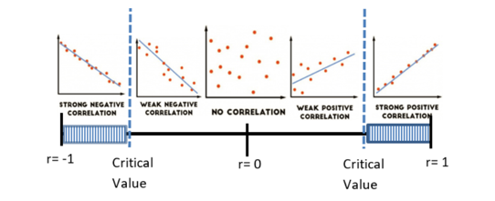
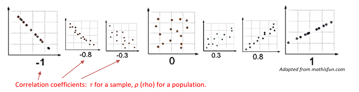
Correlation
Define correlation
Linear Regression
\(\hat y=b+mx\)The regression equation expresses a relationship between x and y.
In the regression equation, what do each of these variables represent?
x:
y:
m:
b:
StatCrunch enter sample data in two columns, then select Stat → Regression → Simple Linear
- Cricket Chirping Frequency and Temperature: Load the chirping frequency data for the striped ground cricket at various ground temperatures. Construct a scatterplot, and run a Regression and Correlation Test using α = 0.01. Determine whether there is sufficient evidence to support a claim of a linear correlation between chirping frequency and ground temperature.
- Claim:
\(\rho \neq 0\) There is a linear correlation between chirping frequency and ground temperature. - \(H_0\) :
\(\rho = 0\) There is no linear correlation. - \(H_A\) :
\(\rho \neq 0\) There is a linear correlation. - Significance level α:
0.01 - p-value (for slope or model)
p < 0.0001 - Decision about the null hypothesis:
\(p<0.0001\) is less than \(α = 0.01\) so Reject \(H_0\) - Concluding Statement:
There is sufficient sample evidence to support the claim of a linear correlation between chirping frequency of the Striped Ground Cricket and ground temperature. - Regression Equation:
\(\hat{y}=26.9 + 1.5x\)
- Is the regression equation a good predictor?
Yes, as long as we stay within the scope of the sample data - Did you reject \(H_0\)?
- The regression line in the scatterplot shows that the line fits the points well.
- Does the correlation coefficient r indicate a linear correlation?
- Is your prediction within the scope of the available data? Or not too much beyond it?
- If you listened in the morning when you woke up and measured a striped ground cricket chirping at a rate of 39 chirps per 15 seconds, how warm would you say the ground temperature is?
\(\hat{y}=26.9+1.5(39) = 85.4\) °F
- If the ground temperature is 78 degrees Fahrenheit, how fast do you predict the crickets to be chirping?
\(78=26.9+1.5x\) x = 34 chirps per 15 seconds
- What is the best predicted ground temperature if crickets are chirping at a rate of 15 chirps every 15 seconds?
Since 15 seconds is not within the scope of the sample data, we cannot rely on the regression equation to make a prediction.
- Claim:
- Exercise and GPA: A student conducts a study to determine whether there is a linear relationship between the number of hours a student exercises each week and the student’s grade point average (GPA). Test the student’s claim at a 0.10 significance level.
Hours of Exercise 12 3 0 6 10 2 18 14 15 5 GPA 3.6 4.0 3.9 2.5 2.4 2.2 3.7 3.0 1.8 3.1
- Claim in words:
There is a linear correlation between hours of exercise and GPA. - Null hypothesis in words:
There is no linear correlation. - Alternate hypothesis in words:
There is a linear correlation. - Significance level α:
0.01 - p-value (for slope or model)
0.6509 - Use the p-value to make a conclusion about the usefulness of the least squares regression line and its equation.
Since we fail to reject the null hypothesis, we do not have sufficient evidence to support the claim of a linear correlation between hours of exercise and GPA. Therefore, the regression equation is not useful for making predications. - Find the best predicted GPA for a student who exercises 5 hours per week.
An alternate method of prediction in this case it to average the GPA’s in the sample. \(\bar{y}=3.02\)
- Claim in words:
- Vocabulary Words: A child psychologist estimated the number of vocabulary words in a sample of 12 children. Each child’s age and the number of words in their vocabulary are paired in the table.
Age 1 2 3 4 5 6 3 5 2 4 6 7 Vocab 3 220 540 1100 1620 2600 1250 2200 260 1200 2500 1900
- With a significance level of 0.05, can the psychologist use this data to support the claim of a linear correlation between a child’s age and the number of words in their vocabulary? How do you know?
Yes, because the p-value is <0.001, so we have sufficient sample evidence of a linear correlation. - What is the slope in the regression equation? What does this slope tell us about the relationship between a child’s age and vocabulary?
The slope is 446. According to the sample data, a child gains 446 vocabulary words per year. - What is the y-intercept of the regression line? Is it reasonable to interpret the y-intercept? Why or why not?
The y-intercept is -503. It is not reasonable to interpret this y-intercept because a child cannot have a negative number of words in their vocabulary. - What is the best prediction for the number of words in a child’s vocabulary if the child is 7 years old?
\(\hat{y}=-503+446\left(7\right)=\) 2619 words - How does the observed vocabulary of the 7-year-old in the sample compare with the predicted value for a 7-year-old?
2619 – 1900 = 719 words - The difference between an observed value and the predicted value of a dependent variable is called a _________
residual
- With a significance level of 0.05, can the psychologist use this data to support the claim of a linear correlation between a child’s age and the number of words in their vocabulary? How do you know?
- Make a circle outlined with cheerios. Place cheerios along the diameter of the circle. Do not leave space between consecutive cheerios.
- How many cheerios did you use for the diameter of your circle?
- How many cheerios did you use for the circumference of your circle?
- Compile your classroom data and run a regression test to determine if there is a linear correlation between diameter and circumference. What is the p-value for slope?
- What is the slope in the regression equation?
- If your classmate wanted to make a cheerio circle using 20 cheerios for the diameter, how many cheerios do you predict they would need to outline the circle?
- Lemon Imports And Crash Fatality Rates : Listed below are annual data for various years. The data are weights (metric tons) of lemons imported from Mexico and US car crash fatality rates per 100,000 population. Construct a scatterplot, and run a Regression and Correlation Test using α = 0.05. Determine whether there is sufficient evidence to support a claim of a linear correlation between weights of lemon imports from Mexico and US car fatality rates. Source: “The trouble with QSAR (or How I Learned to Stop Worrying and Embrace Fallacy)” by Stephen Johnson, Journal of Chemical Information and Modeling. Vol. 48, No 1).
LEMON IMPORTS (metric tons) 230 266 359 480 534 US CRASH FATALITY RATE (per 100,000 population) 15.9 15.7 15.5 15.3 14.8 - Claim:
\(\rho \neq 0\) There is a linear correlation between lemon imports and car crash fatality rates.
- Claim:
- \(H_0\) :
\(\rho = 0\) There is no linear correlation in the population - \(H_A\) :
\(\rho \neq 0\) There is some linear correlation in the population - Critical Value (from Pearson Correlation Critical Value chart):
\(r_{cv}= ±0.878 \) - Correlation Coefficient:
\(r = -0.9554\) - Is this correlation coefficient in the critical region
Yes - Decision about null hypothesis:
Reject \(H_0\) - Concluding Statement:
There is sufficient sample evidence to support the claim of a linear correlation between weights of lemon imports from Mexica and U.S. car crash fatality rates. - Do the results suggest that imported lemons cause car fatalities?
No. Correlation does not imply causation!