Unit 1 Formula Sheet
Standard Deviation:
\(\sigma=\sqrt{\frac{\Sigma\left(x-\mu\right)^2}N}\)
\(s=\sqrt{\frac{\Sigma\left(x-\bar{x}\right)^2}{n-1}}\)
\(s=\sqrt{\frac{\Sigma\left(x-\bar{x}\right)^2f}{n-1}}\)
Range:
\(\text{Range}=\text{Maximum}-\text{Minimum}\)Class Midpoint:
Class Midpoint = \(\frac{LCL+UCL}2\)Class Width:
Relative Frequency:
\( \text {Relative Frequency} = \frac{ \text {Class Frequency} }{ \text {Sample Size} } = \frac fn \)Variance:
\( \text {variance} = \left( \text {standard deviation} \right)^2\)Mean
\(\mu=\frac{\Sigma x}N\)
\(\bar{x}=\frac{\Sigma x}n\)
\(\bar{x}=\frac{\Sigma xw}{\Sigma w}\)
\(\bar{x}=\frac{\Sigma xf}n\)
Interquartile Range and Outliers
\(IQR=Q_3-Q_1\)
\(Q_1-1.5(IQR)\)
\(Q_3+1.5(IQR)\)
Unit 2 Formula Sheet
Classical (or Theoretical) Probability:
\(P(E)=\frac{ \text {Number of Outcomes in Event E} }{ \text {Total number of outcomes in the sample space }}\)
Empirical (or Statistical) Probability:
\(P(E)=\frac{ \text {Frequency of event E} }{ \text {Total frequency} }=\frac fn\)
Probability of a Complement:
\(P(E')=1-P(E)\)
Probability of occurrence of both events A and B:
\(P(A\; \text {and} \;B)=P(A)\cdot P(\left.B\right|A)\)
\(P(A\; \text {and} \;B)=P(A)\cdot P(B)\) if \(A\; \text {and} \;B\) are independent
Probability of occurrence of either A or B:
\(P(A \; \text {or} \; B)=P(A)\;+\;P(B)\;-\;P(A \; \text {and} \; B)\)
\(P(A\; \text {or} \;B)=P(A)\;+\;P(B)\) if A and B are mutually exclusive
Mean of a Discrete Random Variable:
\(\mu=\Sigma x\;P(x)\)
Variance and Standard Deviation of a Discrete Random Variable:
Variance: \(\sigma^2=\Sigma\left(x-\mu\right)^2\;P(x)\)
Standard Deviation: \(\sigma=\sqrt{\sigma^2}=\sqrt{\Sigma\left(x-\mu\right)^2\;P(x)}\)
Expected Value:
\(E(x)=\mu=\Sigma x\;P(x)\)
Binomial Probability of x successes in n trials:
\(P(x)={}_nC_x\;p^xq^{n-x}=\frac{n!}{(n-x)!x!}p^xq^{n-x}\)
Population Parameters of a Binomial Distribution:
Unit 3 Formula Sheet
z-Score:
Population
\(z=\frac{x-\mu}\sigma\)
Sample
\(z=\frac{x-\bar{x}}{s}\)
Transforming a z-Score to an x-Value:
\(x=\mu+z \cdot \sigma\)
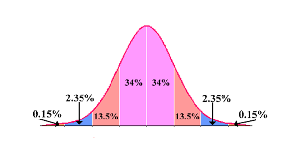
Empirical Rule:
(68-95-99.7 Rule) For symmetric, bell-shaped data sets
Central Limit Theorem:
(\(n\geq30\) or population is normally distributed)
Mean of the Sampling Distribution: \(\mu_x=\mu\)
Standard Deviation of the Sampling Distribution (Standard Error):
\(\sigma_x=\frac\sigma{\sqrt n}\)
z-Score \(=\frac{{\displaystyle\overset\_x}-\mu_x}{\sigma_x}=\frac{\displaystyle\overset\_x-\mu}{ \frac {\sigma}{\sqrt n}}\)
Confidence Interval for the Mean:
\(\overset-x-E<\mu<\overset-x+E\)
\(E=t_c\frac s{\sqrt n}\)
Minimum Sample Size to Estimate the Mean:
\(n=\left(\frac{z_c\sigma}E\right)^2\)
Population Proportion:
\(\widehat p=\frac xn\)
Confidence Interval for Population Proportion:
\(\widehat p-E\;<\;p\;<\;\widehat p+E\)
\(E=z_c\sqrt{\frac{\displaystyle\widehat p\widehat q}n}\)
Minimum Sample Size to Estimate:
\(n=\widehat p\widehat q\left(\frac{z_c}E\right)^2\)
Unit 4 Formula Sheet
Test Statistics:
Mean: \(t=\frac{{\displaystyle\overset\_x}-\mu}{ \frac {s}{\sqrt n}}\)
Proportion: \(z=\frac{{\displaystyle\widehat p}-\mu_{\displaystyle\widehat p}}{\sigma_{\displaystyle\widehat p}}=\frac{\widehat p-p}{\sqrt{ \frac {pq}{n}}}\)
| Null Hypothesis is the Claim | Alternate Hypothesis is the Claim | |
|---|---|---|
| Reject the Null | “There is sufficient sample evidence to reject the claim that…” | “There is sufficient sample evidence to support the claim that…” |
| Fail to Reject the Null | “There is not sufficient sample evidence to reject the claim that…” | “There is not sufficient sample evidence to support the claim that…” |
Correlation Coefficient:
\(r=\frac{n\sum xy-\left(\sum x\right)\left(\sum y\right)}{\sqrt{n\sum x^2-\left(\sum x\right)^2}\sqrt{n\sum y^2-\left(\sum y\right)^2}}\)
t-Test for Linear Correlation:
\(t=\frac r{\sqrt{\displaystyle\frac{1-r^2}{n-2}}}\) (\(\text {degrees of freedom} = n-2\))
Equation of a Regression Line:
\(\widehat y=mx+b\)
| n | Degrees of Freedom | alpha=0.1 | alpha=0.05 | alpha=0.01 |
|---|---|---|---|---|
| 3 | df=1 | 0.988 | 0.997 | 0.999 |
| 4 | df=2 | 0.900 | 0.950 | 0.990 |
| 5 | df=3 | 0.805 | 0.878 | 0.959 |
| 6 | df=4 | 0.729 | 0.811 | 0.917 |
| 7 | df=5 | 0.669 | 0.754 | 0.875 |
| 8 | df=6 | 0.621 | 0.707 | 0.834 |
| 9 | df=7 | 0.584 | 0.666 | 0.798 |
| 10 | df=8 | 0.549 | 0.632 | 0.765 |
| 11 | df=9 | 0.521 | 0.602 | 0.735 |
| 12 | df=10 | 0.497 | 0.576 | 0.708 |
| 13 | df=11 | 0.476 | 0.553 | 0.684 |
| 14 | df=12 | 0.458 | 0.532 | 0.661 |
| 15 | df=13 | 0.441 | 0.514 | 0.641 |
| 16 | df=14 | 0.426 | 0.497 | 0.623 |
| 17 | df=15 | 0.412 | 0.482 | 0.606 |
| 18 | df=16 | 0.400 | 0.468 | 0.590 |
| 19 | df=17 | 0.389 | 0.456 | 0.575 |
| 20 | df=18 | 0.378 | 0.444 | 0.561 |
| 21 | df=19 | 0.369 | 0.433 | 0.549 |
| 22 | df=20 | 0.360 | 0.423 | 0.537 |
| 23 | df=21 | 0.352 | 0.413 | 0.526 |
| 24 | df=22 | 0.344 | 0.404 | 0.515 |
| 25 | df=23 | 0.337 | 0.396 | 0.505 |
| 26 | df=24 | 0.330 | 0.388 | 0.496 |
| 27 | df=25 | 0.323 | 0.381 | 0.487 |
| 28 | df=26 | 0.317 | 0.374 | 0.479 |
| 29 | df=27 | 0.311 | 0.367 | 0.471 |
| 30 | df=28 | 0.306 | 0.361 | 0.463 |
| 31 | df=29 | 0.301 | 0.355 | 0.456 |
| 32 | df=30 | 0.296 | 0.349 | 0.449 |
| 37 | df=35 | 0.275 | 0.325 | 0.418 |
| 42 | df=40 | 0.257 | 0.304 | 0.393 |
| 47 | df=45 | 0.243 | 0.288 | 0.372 |
| 52 | df=50 | 0.231 | 0.273 | 0.354 |
| 62 | df=60 | 0.211 | 0.250 | 0.325 |
| 72 | df=70 | 0.195 | 0.232 | 0.303 |
| 82 | df=80 | 0.183 | 0.217 | 0.283 |
| 92 | df=90 | 0.173 | 0.205 | 0.267 |
| 102 | df=100 | 0.164 | 0.195 | 0.254 |
| 152 | df=150 | 0.134 | 0.159 | 0.208 |
| 302 | df=300 | 0.095 | 0.113 | 0.148 |