Unit 4 Hypothesis Testing
Helper or Hinderer?
Part One - Introduction
Sociology Study from the Yale Infant Cognition Center:
View the Helper or Hinderer Video
Possible response: Maybe 12 to 15 of the infants would choose the helper toy and the rest would choose the hinderer toy.
Example: The infants chose the brighter toy.
Example: The infants chose the softer toy.
Half of the infants would choose the helper toy and half of the infants would choose the hinderer toy.
Possible response: Maybe nine infants would choose the helper toy and 7 infants would choose the hinderer toy.
Yes, because 14 is far higher than half of the number of infants.
Part Two - Exploration
- A key question is, “How surprising is the observed result under the assumption that infants have NO real preference for the helper toy or the hinderer toy?”
- We will call this assumption of no real preference the null hypothesis.
- Let’s simulate this situation using coin flips. If children truly have no preference, they will have a 50/50 chance of picking the helper toy.
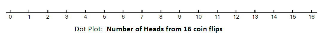
- Flip a coin 16 times. If getting heads represents that the child chose the helper toy, count how many of your 16 hypothetical infants chose the helper toy and place in the blank on the left.(Count the total number of heads from your 16 coin flips.) Repeat this process 3 more times and write the number of heads for each round of 16 in the blanks below.
___________
___________
___________
___________
- Combine your results with your classmates. Do this by producing a dot plot (of the number of infants who choose the helper toy) on the board, where you contribute 4 dots corresponding to your 4 simulations from number 1 above. Copy the class dotplot from the board here below.
- Does it seem like the results actually obtained by these researchers (see number 5 on Part One) would be surprising under the null hypothesis that infants do NOT have a genuine preference for either toy? Explain.
Yes. The coin flipping scenario shows no preference for heads or tails; thus, there is no preference for the helper or hinderer toy.
- Now, we will use technology to simulate completing this experiment many, many times (100, 500, 1000 times) under the assumption that the null hypothesis is true – that infants show no preference of choice over the Helper or Hinderer toy. Based on this simulation, how surprising are the actual results of this study? (Refer back to Part One, number 5). Explain your reasoning.
The results are still quite surprising since the simulation shows that abot 50% of the infants would choose the helper toy, while the other half would choose the hinderer toy.
Part Three - Analysis and Conclusions
There is variability between what we expected to happen, assuming the null hypothesis is true (8 infants choosing helper toy), and the actual results. The question is, “Can the random process of choosing explain this variability, or is there another explanation for this variability?” Many statisticians say that the field of statistics is primarily about explaining variability. This is what we are attempting to do in this investigation, and we will continue to explore these ideas throughout this course.
TERMINOLOGY:
- The probability of an event is the long-run proportion of times the event happens when its random process is repeated indefinitely. It has to do with the likelihood that an event occurs.
- The p-value is the probability that randomness would produce data as (or more) extreme as an actual study, assuming the null hypothesis to be true.
- A small p-value indicates that the observed data would be surprising to occur by randomness alone, if the null hypothesis were true.
- Having results with a small p-value is said to be statistically significant,
- The results did not occur by chance/randomness alone.
- It provides evidence against the null hypothesis.
- Based on our simulations from Part Two, what conclusion should the researchers draw? Justify your conclusions and use the above terminology in your justification.
We would fail to reject the null hypothesis. There is not sufficient evidence to reject the claim that there is no preference in choice of the toy that is chosen.
- If the actual study had instead found that 9 of the 16 infants chose the Helper toy, then what decision should the researchers make based on this result? Justify your conclusions, and use the above terminology in your justification.
We would reject the null hypothesis. There is not sufficient evidence to support the claim that there is no preference in choice of the toy that is chosen.
7.1 Hypothesis Testing with One Sample
Basic Steps of a P-value Hypothesis Test:
Step 1: Write the claim as a mathematical statement.
Step 2: Identify the Null Hypothesis and the Alternative Hypothesis.
Null Hypothesis:
What we assume is true about the population parameter
Will be the same as the claim if the claim contains an equal sign.
\( \left[H_{0}\right] \quad \leq \quad \geq \quad =\)
Always Contains Equality
-
Alternative Hypothesis:
The complement of the null hypothesis
Will be the same as the claim if the claim does not contain an equal sign.
\( \left[H_{A}\right] \quad < \quad > \quad \not=\)
Never Contains Equality
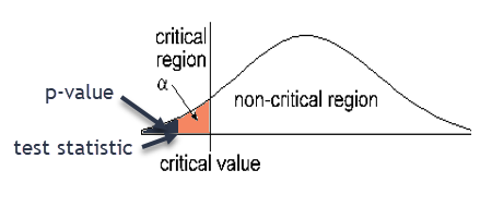
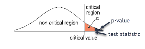
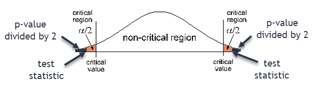
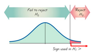
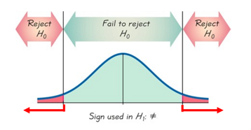
Step 3: Determine the type of test and shade the graph.
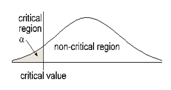
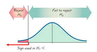
Left- tail: HA contains the following symbol: <
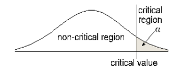
Right-tail: HA contains the following symbol: >
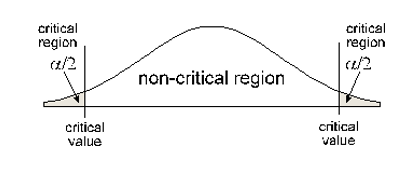
2-tail: HA contains the following symbol: ≠
Rejection area (critical region) is the area beyond your Critical Value and has area α (the significance level of your hypothesis test). In a right or left tail test, that area is in one tail. In a two tail test, the area in each side of the critical region is α/2.Step 4: Calculate the test statistic from sample data.
A Test Statistic is the value computed from sample data and used in making a decision about rejection of the Null Hypothesis.
Test statistic for proportion:
- p = population proportion q = 1 – p
- n = sample size
- \(\hat{p}=\frac{x}{n}\) sample proportion
- \(z=\frac{\hat{p}-p}{\sqrt{\frac{p q}{n}}}\)
Test statistic for mean:
- s = sample standard deviation
- n = sample size
- \(\mu\) = population mean
- \(\overline{x}\) = sample mean
- \(t=\frac{\overline{x}-\mu}{\frac{s}{\sqrt{n}}}\)
Step 5: Calculate the p-value for your test statistic.
P-value: the probability of being as extreme, or more extreme, than your data, assuming the null hypothesis is correct.
- Left tail test: contains “< ”. P-value = area to the left of the test statistic.
- Right tail test: contains “ >”. P-value = area to the right of the test statistic.
- Two tail test: contains “≠”. P-value = twice the area in the tail beyond the test statistic
Step 6: Determine the rejection criteria.
- Using probability: Reject \(H_0\) if the p-value \(\leq\alpha\) .
- Using test statistics: Reject \(H_0\) if the test statistic is in the rejection region.
Step 7: Make One of Two Decisions About the Null Hypothesis
- Reject the Null:
- If P-value \(\leq\alpha\) , reject \(H_0\).
- Type I error: rejecting \(H_0\) when it is actually true
- Fail to Reject the Null:
- If P-value \(> \alpha\), fail to reject \(H_0\).
- Type II error: failing to reject \(H_0\) when it is actually false
Step 8: Make A Statement About The Claim Based On Your Decision About the Null Hypothesis.
| Null is the Claim | Alternate is the Claim | |
|---|---|---|
| Reject the Null | “There is sufficient sample evidence to reject the claim that…” | “There is sufficient sample evidence to support the claim that…” |
| Fail to Reject the Null | “There is not sufficient sample evidence to reject the claim that…” | “There is not sufficient sample evidence to support the claim that…” |
Introduction to Hypothesis Testing: Steps 1-3
Remember to use the correct symbols.
- Mean: \(\mu\)
- Proportion: p
- Standard deviation: \(\sigma\)
- The mean IQ of statistic students is at least 110.
- Claim:
\( \mu \geq 110 \) - \(H_0\):
\( \mu \geq 110 \) (Assume \(H_0: \mu = 110 \)) - \(H_A\):
\( \mu < 110 \) - The significant area (rejection area) is located where
\( \mu \) is significantly less than 110 , therefore, this is aLeft-Tailed test.
- Claim:
- The mean wait time for a GrubHub delivery is more than 40 minutes.
- Claim:
\( \mu > 40 \) - \(H_0\):
\( \mu \leq 40 \) (Assume \(H_0: \mu = 40 \)) - \(H_A\):
\( \mu > 40 \) - The significant area (rejection area) is located where
the mean wait time is significantly greater than 40 minutes , therefore, this is aRight-Tailed test.
- Claim:
- The percentage of people who prefer milk chocolate over dark chocolate is 70% as claimed by Madison advertising agency.
- Claim:
\(p=0.7\) - \(H_0\):
\(p=0.7\) (Assume \(H_0: p=0.7 \)) - \(H_A\):
\(p \neq 0.7\) - The significant area (rejection area) is located where
\(p\) is significantly different than 0.7 , therefore, this is aTwo-Tailed test.
- Claim:
- The percentage of all students who eat sushi at least once per week is less than 27%.
- Claim:
\(p < 0.27\) - \(H_0\):
\(p \geq 0.27\) (Assume \(H_0: p=0.27 \)) - \(H_A\):
\(p < 0.27\) - The significant area (rejection area) is located where
the proportion of all students who eat sushi is significantly less than 27%, , therefore, this is aLeft-Tailed test.
- Claim:
- The mean IQ of statistic students is at most 110.
- Claim:
\( \mu \leq 110 \) - \(H_0\):
\( \mu \leq 110 \) (Assume \(H_0: \mu = 110 \)) - \(H_A\):
\( \mu > 110 \) - The significant area (rejection area) is located where
\( \mu \) is significantly greater than 110 , therefore, this is aRight-Tailed test.
- Claim:
- The percentage of all men who prefer milk chocolate over dark chocolate is different than 70% as claimed by Madison advertising agency.
- Claim:
\(p \neq 0.7\) - \(H_0\):
\(p = 0.7\) - \(H_A\):
\(p \neq 0.7\) (this can be translated ar \(p<0.7\) or \(p>0.7\)) - The significant area (rejection area) is located where
\(p\) is significantly different than 0.7 , therefore, this is aTwo-Tailed test.
- Claim: