Unit 1 Formula Sheet
Chapter 2
Standard Deviation:
Population
\(\sigma=\sqrt{\frac{\Sigma\left(x-\mu\right)^2}N}\)
Sample
\(s=\sqrt{\frac{\Sigma\left(x-\bar{x}\right)^2}{n-1}}\)
Frequency Distribution
\(s=\sqrt{\frac{\Sigma\left(x-\bar{x}\right)^2f}{n-1}}\)
z-Score:
Population
\(z=\frac{x-\mu}\sigma\)
Sample
\(z=\frac{x-\bar{x}}{s}\)
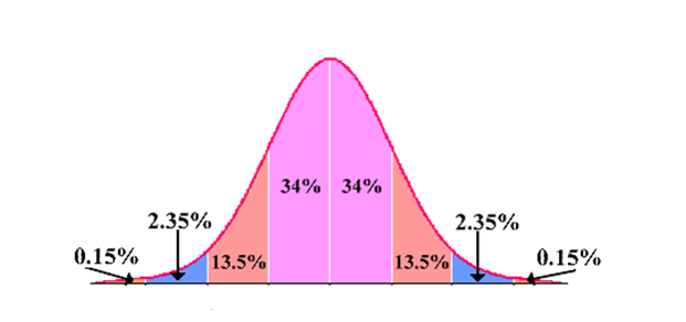
Empirical Rule:
(68-95-99.7 Rule) For symmetric, bell-shaped data sets
Range:
\(\text{Range}=\text{Maximum}-\text{Minimum}\)Class Midpoint:
Class Midpoint = \(\frac{LCL+UCL}2\)Class Width:
From raw data: \(\frac{ \text {Range} }{ \text {Number of Classes} }\) (round up)
From table: \( \text {Class Width} = LCL_2-LCL_1\)
Relative Frequency:
\( \text {Relative Frequency} = \frac{ \text {Class Frequency} }{ \text {Sample Size} } = \frac fn \)Variance:
\( \text {variance} = \left( \text {standard deviation} \right)^2\)Mean
Population
\(\mu=\frac{\Sigma x}N\)
Sample
\(\bar{x}=\frac{\Sigma x}n\)
Weighted
\(\bar{x}=\frac{\Sigma xw}{\Sigma w}\)
Frequency Distribution
\(\bar{x}=\frac{\Sigma xf}n\)
Interquartile Range and Outliers
Interquartile Range
\(IQR=Q_3-Q_1\)
Lower Outlier Critical Value:
\(Q_1-1.5(IQR)\)
Upper Outlier Critical Value:
\(Q_3+1.5(IQR)\)