MATH 1530

Unit 3 Normal Distributions and Confidence Intervals

5.1 Introduction to Normal Distributions and the Standard Normal Distribution

Overview of the Chapter

“If a variable can take on any value between two specified values, it is called a continuous variable; otherwise, it is called a discrete variable. Some examples will clarify the difference between discrete and continuous variables.

• Suppose the fire department mandates that all fire fighters must weigh between 150 and 250 pounds. The weight of a fire fighter would be an example of a continuous variable; since a fire fighter's weight could take on any value between 150 and 250 pounds.
• Suppose we flip a coin and count the number of heads. The number of heads could be any integer value between 0 and infinity. However, it could not be any number between 0 and infinity. We could not, for example, get 2.5 heads. Therefore, the number of heads must be a discrete variable.

Just like variables, probability distributions can be classified as discrete or continuous. A continuous probability distribution differs from a discrete probability distribution in several ways.

• The probability that a continuous random variable will assume a particular value is zero.
• As a result, a continuous probability distribution cannot be expressed in tabular form.
• Instead, an equation or formula is used to describe a continuous probability distribution.

Most often, the equation used to describe a continuous probability distribution is called a probability density function. Sometimes, it is referred to as a density function, a PDF, or a pdf. For a continuous probability distribution, the density function has the following properties:

• Since the continuous random variable is defined over a continuous range of values (called the domain of the variable), the graph of the density function will also be continuous over that range.
• The area bounded by the curve of the density function and the x-axis is equal to 1, when computed over the domain of the variable.
• The probability that a random variable assumes a value between a and b is equal to the area under the density function bounded by a and b.”

Stattrek.com

Three Normal Distributions We Will Use in this Chapter

Standard Normal Bell Curve: a distribution of z-scores

\(\sim \mathbf{N}(\mathbf{0}, \mathbf{1})\)

This is a standardized normal bell curve and is a distribution of z scores. The distribution of z-scores always has the same mean and standard deviation.

Normal Bell Curve: a distribution of individual values

\(\sim \mathbf{N}(\mu, \sigma) \quad z=\frac{x-\mu}{\sigma}\)

This is a normal bell curve and is a distribution of individual x values which are measures for each member of the population. The mean and standard deviation will vary for each population.

Central Limit Theorem Normal Bell Curve: a distribution of sample means

\(\sim \mathbf{N}\left(\mu, \frac{\sigma}{\sqrt{n}}\right) \quad z_{x}=\frac{\overline{x}-\mu}{\left(\frac{\sigma}{\sqrt{n}}\right)}\)

Requirements for CLT:

Sample is from normally distributed population OR Sample size is greater than 30 ( n > 30 )

Properties of a Normal Distribution

In this chapter, you will begin to study the most important continuous probability distribution in statistics: The Normal Distribution. In the previous chapter, discrete distributions could be graphed with a histogram. For continuous probability distributions, we will use a probability density function.

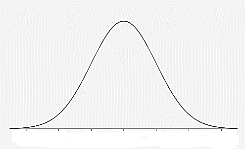
Probability density curve for a normal distribution:

• The mean, median and mode are equal.
• The normal curve is bell shaped and is symmetric about the mean.
• The total area underneath the curve is equal to 1.
• The normal curve approaches, but never touches, the x-axis as it extends away from the mean.
• Between z=-1 and z=1, the graph curves downward. Everywhere else, the graph curves upward.

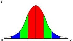
Empirical Rule Review

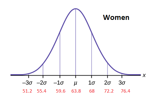
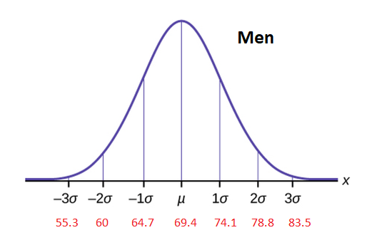
The distribution of the height of American women can be described by a normal curve with a mean \(\mu=63.8\) inches and a standard deviation \(\sigma=4.2\) inches. The distribution for men has a mean \(\mu=69.4\) inches and a standard deviation \(\sigma=4.7\) inches.

Label the curves with x values, z-scores, and estimated probabilities.










1. To join the Boston Beanstalks, a social club for tall people, women must be at least 5 feet 10 inches (70 inches) and men at least 6 feet 2 inches (74 inches).
   
   1. Calculate the z-score for the qualifying height for women to join the Boston Beanstalks.

      \(z=\frac{70-63.8}{4.2}=1.4762\)

   2. Calculate the z-score for the qualifying height for men.

      \(z=\frac{74-69.4}{4.7}=0.979\)

2. Based on the 68-95-99.7% Rule (using z-table or StatCrunch):
   1. Approximately what percentage of American men are tall enough to join the Boston Beanstalks? approximately 16%
   2. Approximately what percentage of American women are tall enough to join the club? approximately 10.5%

Interpreting the Graphs of Normal Curves

Estimating standard deviation based on the point of inflection:

Estimate the standard deviation of the distribution:

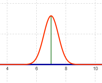
\(\sigma \approx 0.5\)

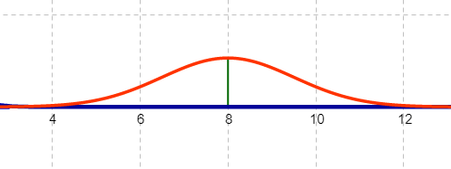
\(\sigma \approx 1.5\)